

Robotic Arm Simulation
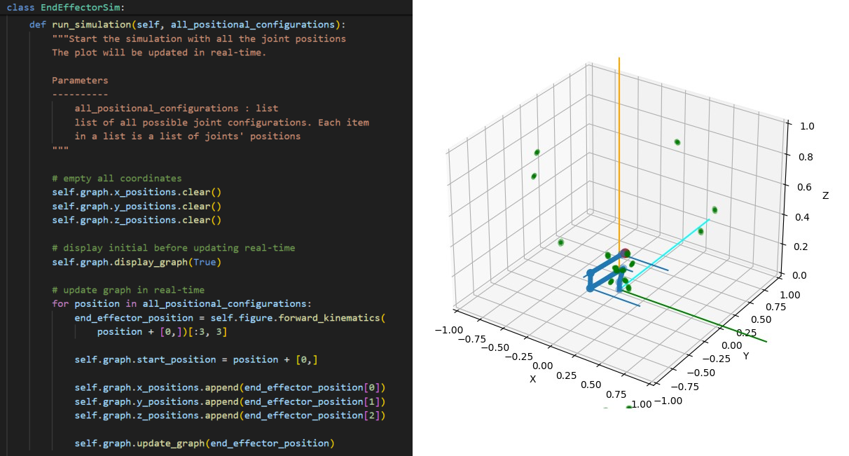
A simulation that plots all possible reachable points for a robotics arm.
Timeline
August 2023 – September 2023
Implementation Details
Programming Language: Python.
Libraries: PyBullet, Ikpy, Matplotlib, and NumPy.
Associated with: TrickFire Robotics
Link to GitHub repository: Robotics Arm Workspace Simulation
Overview
The current arm for our rover weighs a lot, which makes the rover overweight according to the URC competition rule. So, we aimed to redesign and optimize the arm.
To do this, we need to figure out the possible reachable points for the arm, this is called the arm's “workspace”. The mechanical team will then use this data to come up with the best possible re-design for the arm.
Goals
- Develop a simulation that can plot the arm's reachable points given the unified robotics description format (URDF) file.
- Plot the reachable points (discrete) on a 3D graph.
Planning
I picked up the code from a previous team member who already graduated. However, the original code used a controller to move the model of the arm to the target position, so I needed to refactor the code and write my own logic for the arm to automatically reach every possible position it can reach in space and plot that into a graph.
Tasks Checklist:
- Understand the code written by the previous member.
- Figure out ways to get to every possible point the arm can reach.
- Plot each point on a 3D graph.
- Testing with a lower degree of freedom (DOF) arm first.
- Restructure code into class(es) for reusability.
- Test with the current arm URDF file.
- Documentation
Research:
Select libraries:
- PyBullet - To get the “joint” information.
- Ikpy - Compute forward and inverse kinematics algorithms.
- NumPy - Generate a set of discrete points in between each joint's maximum and minimum limit. Compute permutation (generate all possible joint configurations) with the given points.
- Matplotlib - Graphing utility. Plot points on a 3D graph
Class Design (Description)
- Class Graph: Display a 3D graph of all reachable points with the input figure and scatter points.
- Class EndEffectorSim: run the simulation. Each joint has a certain joint limit defined in the .urdf file. Based on that, permutation is used to generate a list of all possible joint positions (given a certain precision). Then, forward kinematics is used to calculate the end effector position.
Note:
Depending on the input precision, the distance between points would be sparse or dense. For example, for a joint limit between 0 and pi radian, if the precision is 3, 3 points will be generated inclusively (e.g. 0, 0.5 pi, and pi). Of course, the more precision, the better. But since joints' position need to be in a specific order, permutation is used. Thus, more precision = slower run time.
Outcomes
There are 2 modes:
- Plot all reachable points: plot reachable points on the graph with the model.
- Real-time simulation: update the graph as the new point is generated.
Real-Time Simulation:
A note on precision:
Depending on how "precise" or "close" you want your points to be. But more points don't always mean better visualization. Increasing the precision slows calculation time since possible configurations are calculated using permutation. Additionally, too high precision can cluster your 3D graph.
For each graph below, notice that less precision = less dense. But the reachable points are sparse and it is difficult to visualize the reachable positions. Since the alpha of each scatter point is set to 0.1, the transparency of a point indicates the frequency of that point being reached. A solid point means that it has been reached multiple times. Likewise, an almost-transparent point shows that the arm only reaches it once or twice.
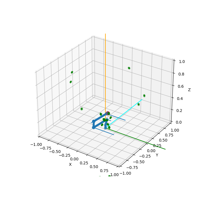
Example of a precision = 3 plot
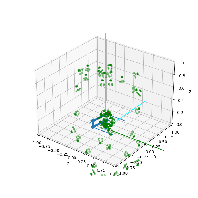
Example of a precision = 4 plot
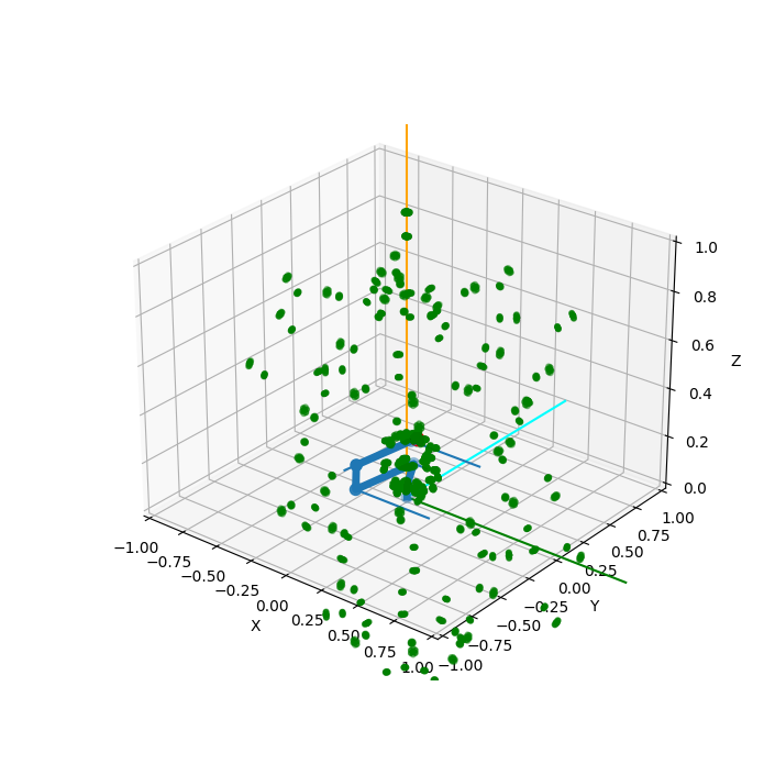
Example of a precision = 5 plot
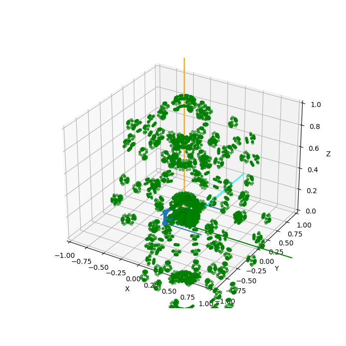
Example of a precision = 6 plot